Overfitting and Data Splitting

Tyler George

Cornell College
DSC 223 - Spring 2024 Block 7

Goals

• Overfitting
• Data splitting to avoid overfitting

Setup

library(tidyverse)
library(tidymodels)
library(gghighlight)
library(kableExtra)
set.seed(1234)

Data and exploration

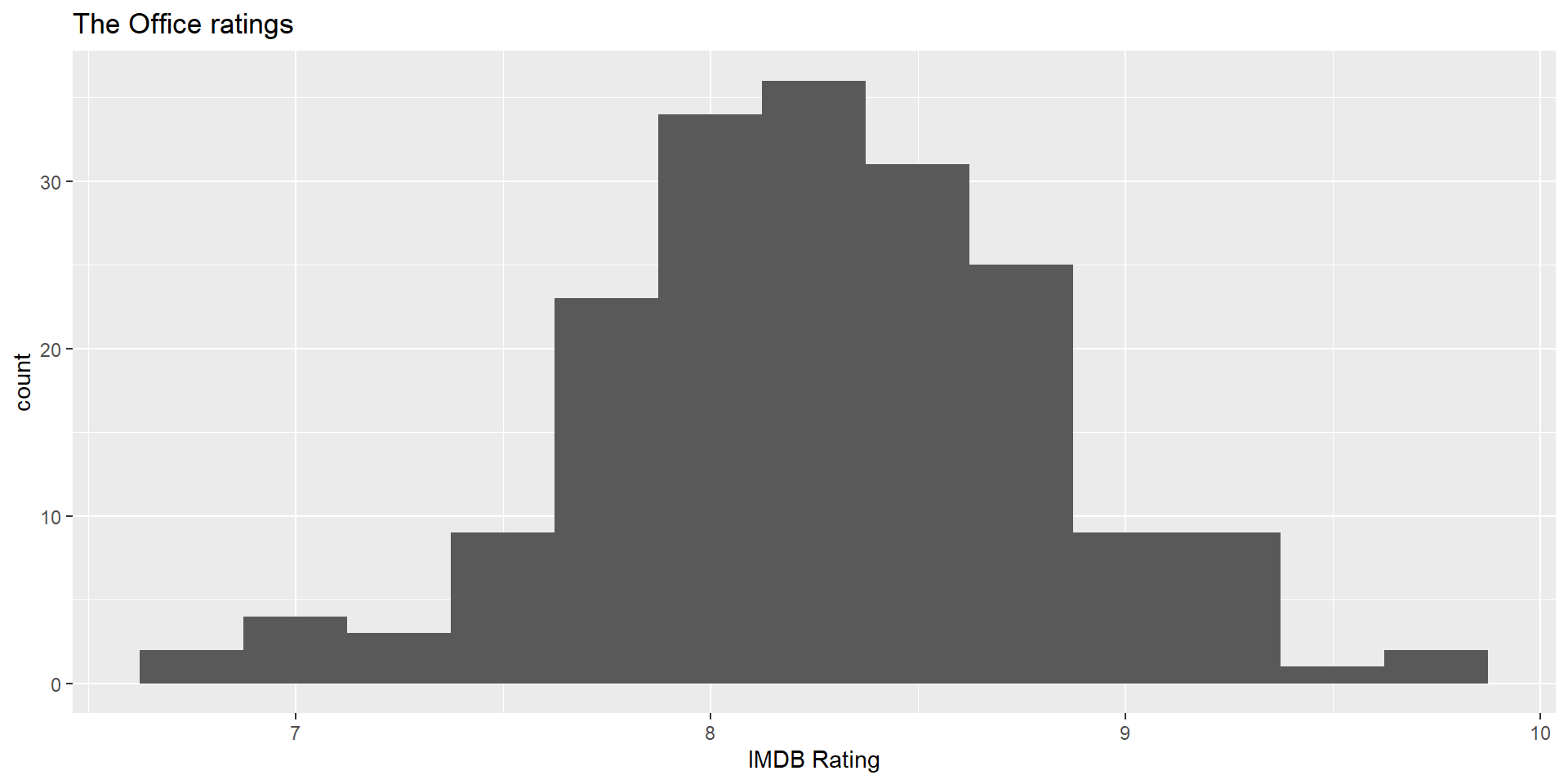
Data

office_ratings <- read_csv("data/office_ratings.csv")
office_ratings

# A tibble: 188 × 6
   season episode title             imdb_rating total_votes air_date  
    <dbl>   <dbl> <chr>                   <dbl>       <dbl> <date>    
 1      1       1 Pilot                     7.6        3706 2005-03-24
 2      1       2 Diversity Day             8.3        3566 2005-03-29
 3      1       3 Health Care               7.9        2983 2005-04-05
 4      1       4 The Alliance              8.1        2886 2005-04-12
 5      1       5 Basketball                8.4        3179 2005-04-19
 6      1       6 Hot Girl                  7.8        2852 2005-04-26
 7      2       1 The Dundies               8.7        3213 2005-09-20
 8      2       2 Sexual Harassment         8.2        2736 2005-09-27
 9      2       3 Office Olympics           8.4        2742 2005-10-04
10      2       4 The Fire                  8.4        2713 2005-10-11
# ℹ 178 more rows

Source: The data come from data.world, by way of TidyTuesday.

IMDB ratings

• Code
• Plot

imbd_hist<-
  ggplot(office_ratings, aes(x = imdb_rating)) +
  geom_histogram(binwidth = 0.25) +
  labs(
    title = "The Office ratings",
    x = "IMDB Rating"
  )

imbd_hist

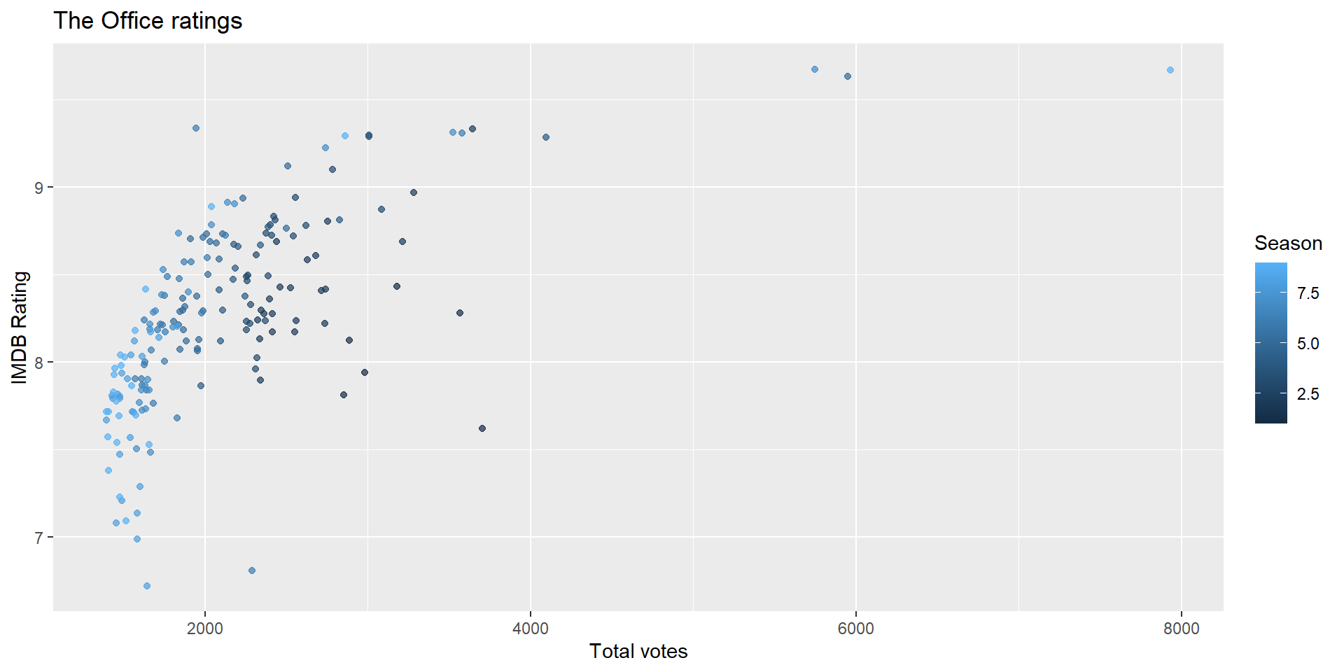
IMDB ratings vs. number of votes

• Code
• Plot

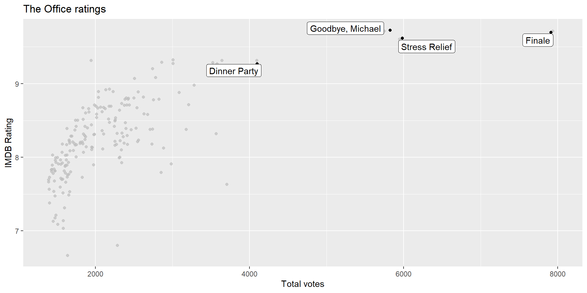
rat_vs_vote_plot<-
  ggplot(office_ratings, aes(x = total_votes, 
       y = imdb_rating, color = season)) +
  geom_jitter(alpha = 0.7) +
  labs(
    title = "The Office ratings",
    x = "Total votes",
    y = "IMDB Rating",
    color = "Season"
  )

rat_vs_vote_plot

Outliers

• Code
• Plot

outlier_plot<- 
  ggplot(office_ratings, 
         aes(x = total_votes, y = imdb_rating)) +
  geom_jitter() +
  gghighlight(total_votes > 4000, label_key = title) +
  labs(
    title = "The Office ratings",
    x = "Total votes",
    y = "IMDB Rating"
  )

If you like the Dinner Party episode, I highly recommend this “oral history” of the episode published on Rolling Stone magazine.

outlier_plot

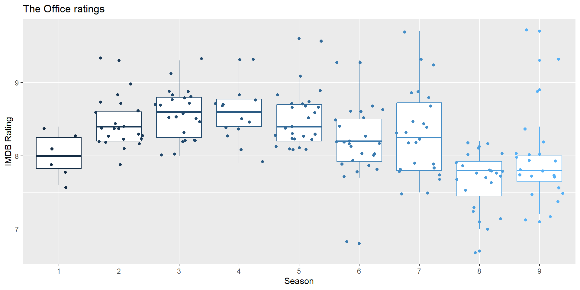
IMDB ratings vs. seasons

• Code
• Plot

rat_sea_box<-
  ggplot(office_ratings, 
         aes(x = factor(season), 
             y = imdb_rating, color = season)) +
  geom_boxplot() +
  geom_jitter() +
  guides(color = "none") +
  labs(
    title = "The Office ratings",
    x = "Season",
    y = "IMDB Rating"
  )

rat_sea_box

Modeling

Train / test

• Create an initial split

set.seed(1122)
office_split <- initial_split(office_ratings) # prop = 3/4 by default

• Save training data

office_train <- training(office_split)
dim(office_train)

[1] 141   6

• Save testing data

office_test  <- testing(office_split)
dim(office_test)

[1] 47  6

Specify model

office_mod <- linear_reg() |>
  set_engine("lm")

office_mod

Linear Regression Model Specification (regression)

Computational engine: lm 

Build recipe

office_rec <- recipe(imdb_rating ~ ., data = office_train) |>
  # title isn't a predictor, but keep around to ID
  update_role(title, new_role = "ID") |>
  # extract month of air_date
  step_date(air_date, features = "month") |>
  step_rm(air_date) |>
  # make dummy variables of month
  step_dummy(contains("month")) |>
  #remove zero variance predictors
  step_zv(all_predictors())

office_rec

── Recipe ────────────────────────────────────────────────────────────────────────────────

── Inputs 

Number of variables by role

outcome:   1
predictor: 4
ID:        1

── Operations 

• Date features from: air_date

• Variables removed: air_date

• Dummy variables from: contains("month")

• Zero variance filter on: all_predictors()

Build workflow

office_wflow <- workflow() |>
  add_model(office_mod) |>
  add_recipe(office_rec)

office_wflow

══ Workflow ══════════════════════════════════════════════════════════════════════════════
Preprocessor: Recipe
Model: linear_reg()

── Preprocessor ──────────────────────────────────────────────────────────────────────────
4 Recipe Steps

• step_date()
• step_rm()
• step_dummy()
• step_zv()

── Model ─────────────────────────────────────────────────────────────────────────────────
Linear Regression Model Specification (regression)

Computational engine: lm 

Fit model

office_fit <- office_wflow |>
  fit(data = office_train)

tidy(office_fit) |>
  print(n = 8)

# A tibble: 12 × 5
  term                estimate std.error statistic  p.value
  <chr>                  <dbl>     <dbl>     <dbl>    <dbl>
1 (Intercept)         7.23     0.205        35.4   3.14e-68
2 season             -0.0499   0.0157       -3.18  1.86e- 3
3 episode             0.0353   0.0101        3.50  6.44e- 4
4 total_votes         0.000352 0.0000448     7.85  1.39e-12
5 air_date_month_Feb  0.0242   0.147         0.165 8.69e- 1
6 air_date_month_Mar -0.145    0.144        -1.01  3.16e- 1
7 air_date_month_Apr -0.106    0.140        -0.759 4.49e- 1
8 air_date_month_May  0.0575   0.175         0.329 7.43e- 1
# ℹ 4 more rows

Evaluate model

Make predictions for training data

office_train_pred <- predict(office_fit, office_train) |>
  bind_cols(office_train |> select(imdb_rating, title))

office_train_pred

# A tibble: 141 × 3
   .pred imdb_rating title               
   <dbl>       <dbl> <chr>               
 1  7.90         8.1 Garden Party        
 2  8.43         7.9 The Chump           
 3  7.81         7.1 Here Comes Treble   
 4  7.94         6.7 Get the Girl        
 5  7.92         7.9 Tallahassee         
 6  8.29         7.7 The Inner Circle    
 7  7.95         7.8 The Sting           
 8  8.00         7.8 WUPHF.com           
 9  9.56         9.6 Stress Relief       
10  8.11         8.1 Manager and Salesman
# ℹ 131 more rows

R-squared

Percentage of variability in the IMDB ratings explained by the model

rsq(office_train_pred, truth = imdb_rating, estimate = .pred)

# A tibble: 1 × 3
  .metric .estimator .estimate
  <chr>   <chr>          <dbl>
1 rsq     standard       0.500

Question: Are models with high or low \(R^2\) more preferable?

RMSE

An alternative model performance statistic: root mean square error

\[ RMSE = \sqrt{\frac{\sum_{i = 1}^n (y_i - \hat{y}_i)^2}{n}} \]

rmse(office_train_pred, truth = imdb_rating, estimate = .pred)

# A tibble: 1 × 3
  .metric .estimator .estimate
  <chr>   <chr>          <dbl>
1 rmse    standard       0.373

Question: Are models with high or low RMSE are more preferable?

Interpreting RMSE

Question: Is this RMSE considered low or high? ]

office_train |>
  summarise(min = min(imdb_rating), max = max(imdb_rating))

# A tibble: 1 × 2
    min   max
  <dbl> <dbl>
1   6.7   9.7

but, really, who cares about predictions on training data?

Make predictions for testing data

office_test_pred <- predict(office_fit, office_test) |>
  bind_cols(office_test |> select(imdb_rating, title))

office_test_pred

# A tibble: 47 × 3
   .pred imdb_rating title               
   <dbl>       <dbl> <chr>               
 1  8.52         8.4 Office Olympics     
 2  8.54         8.6 The Client          
 3  8.90         8.8 Christmas Party     
 4  8.71         9   The Injury          
 5  8.50         8.2 Boys and Girls      
 6  8.46         8.4 Dwight's Speech     
 7  8.64         8.9 Gay Witch Hunt      
 8  8.35         8   Diwali              
 9  8.77         8.7 A Benihana Christmas
10  8.40         8.2 Ben Franklin        
# ℹ 37 more rows

Evaluate performance on testing data

• RMSE of model fit to testing data

rmse(office_test_pred, truth = imdb_rating, estimate = .pred)

# A tibble: 1 × 3
  .metric .estimator .estimate
  <chr>   <chr>          <dbl>
1 rmse    standard       0.386

• \(R^2\) of model fit to testing data

rsq(office_test_pred, truth = imdb_rating, estimate = .pred)

# A tibble: 1 × 3
  .metric .estimator .estimate
  <chr>   <chr>          <dbl>
1 rsq     standard       0.556

Training vs. testing

metric	train	test	comparison
RMSE	0.373	0.386	RMSE lower for training
R-squared	0.500	0.556	R-squared higher for training

Evaluating performance on training data

• The training set does not have the capacity to be a good arbiter of performance.

• It is not an independent piece of information; predicting the training set can only reflect what the model already knows.

• Suppose you give a class a test, then give them the answers, then provide the same test. The student scores on the second test do not accurately reflect what they know about the subject; these scores would probably be higher than their results on the first test.

Source: tidymodels.org